Three-Dimensional Standard Configuration 10
A three-dimensional Standard Configuration 10 test case was proposed by Matthew Montgomery and Joe Verdon in their paper A Three-Dimensional Linearized Unsteady Euler Analysis for Turbomachinery Blade Rows. Ralf Kemme also performed inviscid simulation of this test which he reported in his thesis Numerical Investigation of the Aeroelastic Stability Behaviour of a Highly Loaded Compressor Rotor. RPMTurbo has performed inviscid and viscous simulations of this test case and the results are reported below.
Geometry
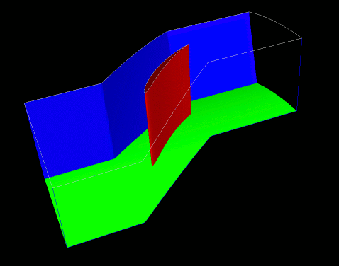
The three-dimensional Standard Configuration 10 test case consists of 24 evenly spaced straight blades. The cross-section of the blades is the same as the two-dimensional Standard Configuration 10 test case. The leading edges of the blades are on straight lines radiating out from the axis which are in the same axial plane. The radius of the hub is 3.395 chord lengths and the radius of the shroud is at 4.244 chord lengths. There is no tip clearance. For the viscous simulations, the chord length was set to 100 mm.

Steady-State Flow
The flow conditions were chosen to match the subsonic case for two-dimensional Standard Configuration 10. It was assumed that the compressor blades are not rotating and that the inlet conditions did not vary with radius. The flow conditions used for the 3D simulations are shown in the Table below.
| Total Pressure | 101.3 kPa |
|---|---|
| Total Temperature | 300.0 K |
| Inflow Angle | 55.0 degrees |
| Inlet Mach Number | 0.7 |
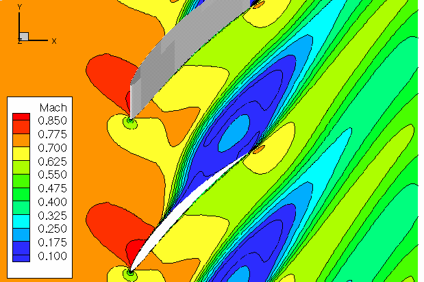
Significant flow blockage due to corner separation at the hub on the suction surface was predicted by the 3D viscous simulation. The corner separation can be seen below in the contour plot of flow Mach Number at ten percent blade height. As a result of this flow blockage, a significantly lower average back pressure, 81.2 kPa, was required for the 3D viscous simulation to achieve an average inlet Mach number of 0.7 compared with the back pressure, 87.26 kPa, requried for the 2D viscous simulation.

The flow conditions used here are slightly different to those used by previous researchers (Montgomery & Verdon and Kemme). They assumed that the blades were rotating and that the relative inflow angle varied with radius. The previous researchers only performed inviscid simulations and achieved good agreement between the 2D and 3D solutions. The flow conditions used here were modified in an attempt to reduce the amount of flow blockage in the 3D viscous simulation.
The RPMTurbo solutions are shown in the Table below. Click on any figure to see a larger view.
| radius / height | Cp Plot |
Isentropic Mach Number Plot |
Friction Coefficient |
Euler Solution | Viscous Solution |
|---|---|---|---|---|---|
| 0.1 |
 |
 |
 |
[Data] | [Data] |
| 0.2 |
 |
 |
 |
[Data] | [Data] |
| 0.3 |
 |
 |
 |
[Data] | [Data] |
| 0.4 |
 |
 |
 |
[Data] | [Data] |
| 0.5 |
 |
 |
 |
[Data] | [Data] |
| 0.6 |
 |
 |
 |
[Data] | [Data] |
| 0.7 |
 |
 |
 |
[Data] | [Data] |
| 0.8 |
 |
 |
 |
[Data] | [Data] |
| 0.9 |
 |
 |
 |
[Data] | [Data] |
Unsteady Flow
The unsteady flow response due to pitching about (0.5, 0.05) in profile co-ordinates is shown in the Table below. The mode shape does not vary with radius, that is the blade slides over the hub and the shroud. The reduced frequency based on full chord is 0.5 and the interblade phase angle is 0 degrees.
| radius/height | Unsteady Cp Plot | Local Work Coefficient |
Euler data | Viscous data |
|---|---|---|---|---|
| 0.1 |
 |
 |
[Data] | [Data] |
| 0.2 |
 |
 |
[Data] | [Data] |
| 0.3 |
 |
 |
[Data] | [Data] |
| 0.4 |
 |
 |
[Data] | [Data] |
| 0.5 |
 |
 |
[Data] | [Data] |
| 0.6 |
 |
 |
[Data] | [Data] |
| 0.7 |
 |
 |
[Data] | [Data] |
| 0.8 |
 |
 |
[Data] | [Data] |
| 0.9 |
 |
 |
[Data] | [Data] |
Aerodynamic Damping
The aerodynamic damping as a function of interblade phase angle for a pitching mode at a reduced frequency of 0.5 is shown in the Table below.
| Mode | ω* | Plot | Data |
|---|---|---|---|
| pitching | 0.5 |
 |
[Data] |